Transformer Encoder Explained

I've recently been spending a lot of spare time digging into the ins and outs of the ever so interesting space of Machine Learning. Started out with the fantastic "Dive into Deep Learning" book, through countless blog posts all over the internet, to "Generative AI System Design Interview" by Ali Aminian and Hao Sheng.

Then, one day while browsing X, I noticed that there was a lot of emphasis being put by the ML community on actually implementing research papers from scratch in order to actually understand the whole concept, and to test oneself in actually understanding every last bit of the math and methods being presented in the publication. This makes a lot of sense, obviously. There is a popular saying that is relevant to this: “In theory, there is no difference between theory and practice; in practice, there is”. Very well then I thought, let's jump into the implementation.

The first thing I had to do was to find the paper to implement. It was all but a short think that followed, and naturally my decision to implement one of the most important papers of the recent times: "Attention Is All You Need" by Vaswani et al. That paper gave birth to the age of LLMs, which I believe might turn out to be the start of the next Industrial Revolution. Except this time we might call it the AI revolution.

The paper introduced the concept of Transformers -- a new attention-based network architecture, which came to be the most important innovation of the past few years. In the paper, The transformer architecture is depicted as follows:

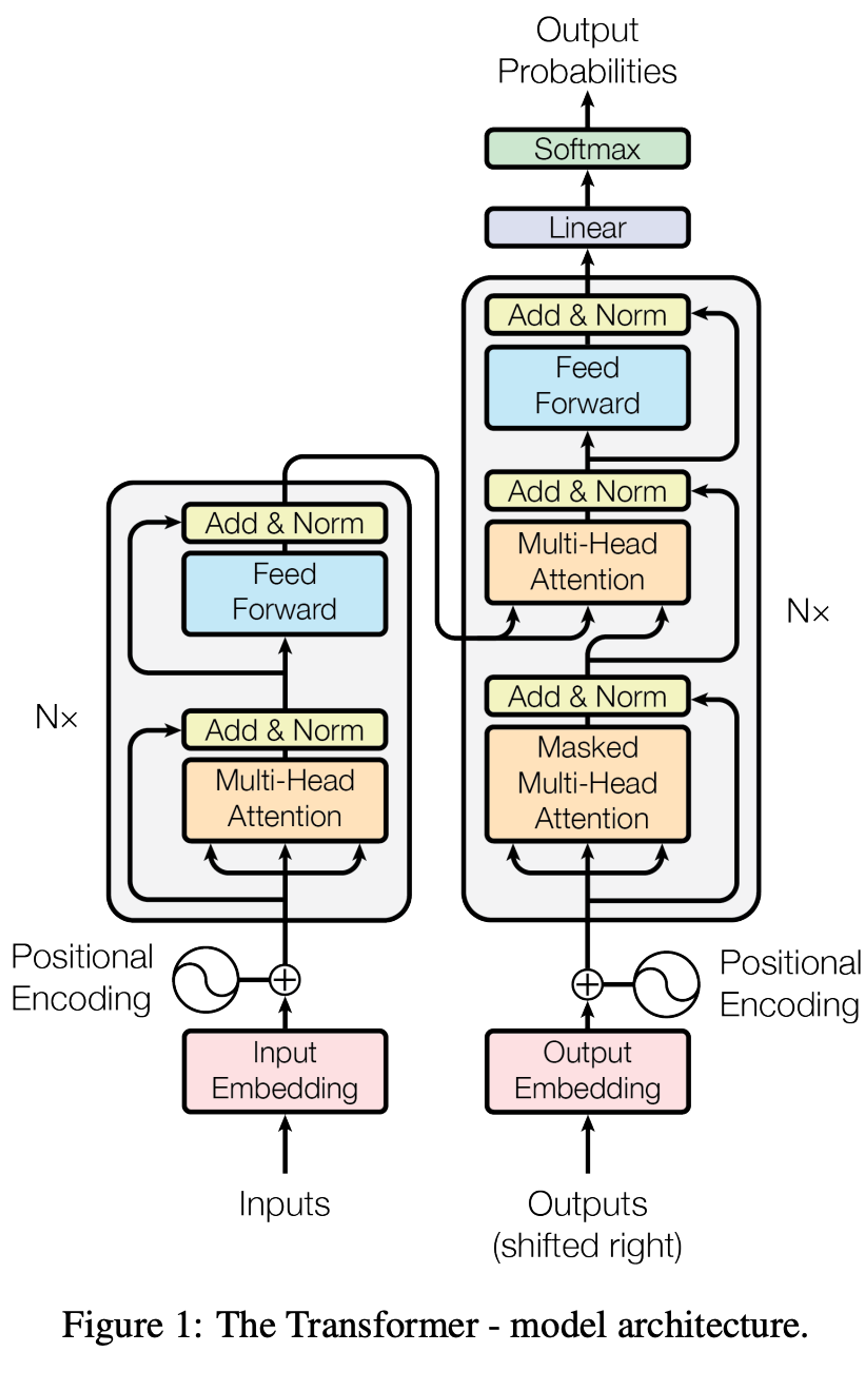
In practice, this is the architecture of the entire encoder-decoder, sequence-to-sequence model that was trained as part of the research. The left side is the encoder. The right side is the decoder. Simple, right?

Let's unpack this step by step first.

The goal of the network presented in the paper is to translate sentences. It transforms one sequence to another. The encoder first produces a latent embedding -- it encodes the text to an internal, numeric representation. The decoder re-interprets that chain of numbers into the sentence in the target language. That's the high level concept.

In this venture, we're only going to implement the encoder.

Let’s define it!

class Encoder(nn.Module):
    def __init__(
        self,
        vocab_size: int,
        d_model: int = 512,
    ):
        super().__init__()
        self.d_model = d_model

Starting simple.

Next, we will handle the input transformations. In the paper, authors define two key components: Input Embedding and Positional Encoding. The concept is text -> tokens -> embeddings (through input embedding) + positional encoding = input to the first Transformer block. The Input Embedding is basically a matrix of learned values.

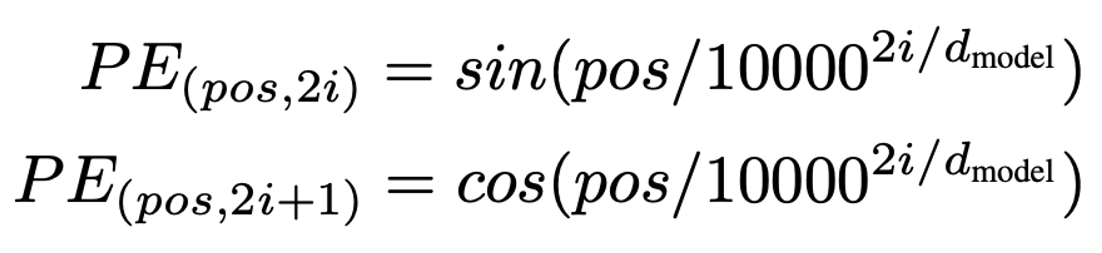
The Positional Encoding is a bit more complex. It’s a way to represent the token positions through sine and cosine transformations, in order to let the model easily learn to attend to relative positions. The authors also stated that learned positional embeddings are nearly identical in performance. Nevertheless, they decided to go with since and cosine transformations. They hypothesized that it’ll allow the model to extrapolate to longer sequences than those seen during training. Formally, it is defined as:

Let's code this! Luckily enough, we can resort to some existing building blocks offered by PyTorch. More concretely, the Input (token) Embedding is very simple to add. We can do it by resorting to the “nn.Embedding” class like so:

        ...
        self.d_model = d_model
        self.token_embedding = nn.Embedding(vocab_size, d_model)

Subsequently, we define the Positional Encoding function.

    # x is [batch, seq_len, d_model]
    # PE(pos,2i)   = sin(pos/10000^(2i/dmodel))
    # PE(pos,2i+1) = cos(pos/10000^(2i/dmodel))
    def get_pos_encoding(self, x: torch.Tensor):
        seq_len = x.size(1)
 
        # [seq_len, 1]
        pos = torch.arange(seq_len, dtype=x.dtype, device=x.device).unsqueeze(1)
        # [d_model / 2]
        i = torch.arange(0, self.d_model, 2, dtype=x.dtype, device=x.device)
        div_term = torch.exp(i * -(math.log(10000.0) / self.d_model))
 
        pos_encoding = torch.zeros(seq_len, self.d_model, dtype=x.dtype, device=x.device)
        pos_encoding[:, 0::2] = torch.sin(pos * div_term)
        pos_encoding[:, 1::2] = torch.cos(pos * div_term)
 
        return pos_encoding.unsqueeze(0)

This is probably the trickiest part of the whole implementation, because it involves several tensor-manipulation steps. Let's go over it very briefly.

Our input "x" is a tensor with shape [batch, seq_len, d_model].

• batch: lets us process multiple examples at once for efficient GPU use
• seq_len: the maximum number of tokens in each sequence
• d_model: the size of each token’s embedding (the model’s hidden dimension)

Next, we create two helper tensors:

• pos - the position of each token in the sequence
• i - the indices of the embedding dimensions (the even ones)

Using these, we compute div_term, which assigns a unique frequency to each embedding dimension. This is how the sinusoidal positional encoding works: different dimensions "wiggle" at different speeds.

Finally, we use pos, i, and div_term to fill in the sine and cosine values that form the full positional encoding matrix.

Okay, that was some heavy math. We can take a breather now. We have the first part of the encoder, and we can combine our Input and Positional Embedding:

class Encoder(nn.Module):
 
    def __init__(
        self,
        vocab_size: int,
        d_model: int = 512,
        n_layers: int = 6,
    ):
        super().__init__()
 
        self.d_model = d_model
        self.token_embedding = nn.Embedding(vocab_size, d_model)
 
    def forward(self, token_ids: torch.Tensor):
        embeddings = self.token_embedding(token_ids)
 
        # From the paper:
        # In the embedding layers, we multiply those weights by √dmodel.
        embeddings = embeddings * math.sqrt(self.d_model)
 
        pos_encoding = self.get_pos_encoding(embeddings)
        in_embeddings = embeddings + pos_encoding
 
    def get_pos_encoding(self, x: torch.Tensor):
        seq_len = x.size(1)
 
        pos = torch.arange(seq_len, dtype=x.dtype, device=x.device).unsqueeze(1)
        i = torch.arange(0, self.d_model, 2, dtype=x.dtype, device=x.device)
        div_term = torch.exp(i * -(math.log(10000.0) / self.d_model))
 
        pos_encoding = torch.zeros(seq_len, self.d_model, dtype=x.dtype, device=x.device)
        pos_encoding[:, 0::2] = torch.sin(pos * div_term)
        pos_encoding[:, 1::2] = torch.cos(pos * div_term)
 
        return pos_encoding.unsqueeze(0)

As the paper suggests, we first get the token embeddings, then position encodings. We sum them together et voila! We have the input!

Now hold on a second -- what's that?

embeddings = embeddings * math.sqrt(self.d_model)

If you read carefully through the entire paper, you'll find this excerpt about how they handle embeddings:

The goal being to scale the embeddings to a similar distribution as the Positional Encodings. Otherwise, the Input Embeddings would dominate, and the training would not be stable!

With that out of the way, we can proceed to the crème de la crème -- the Transformer block itself.

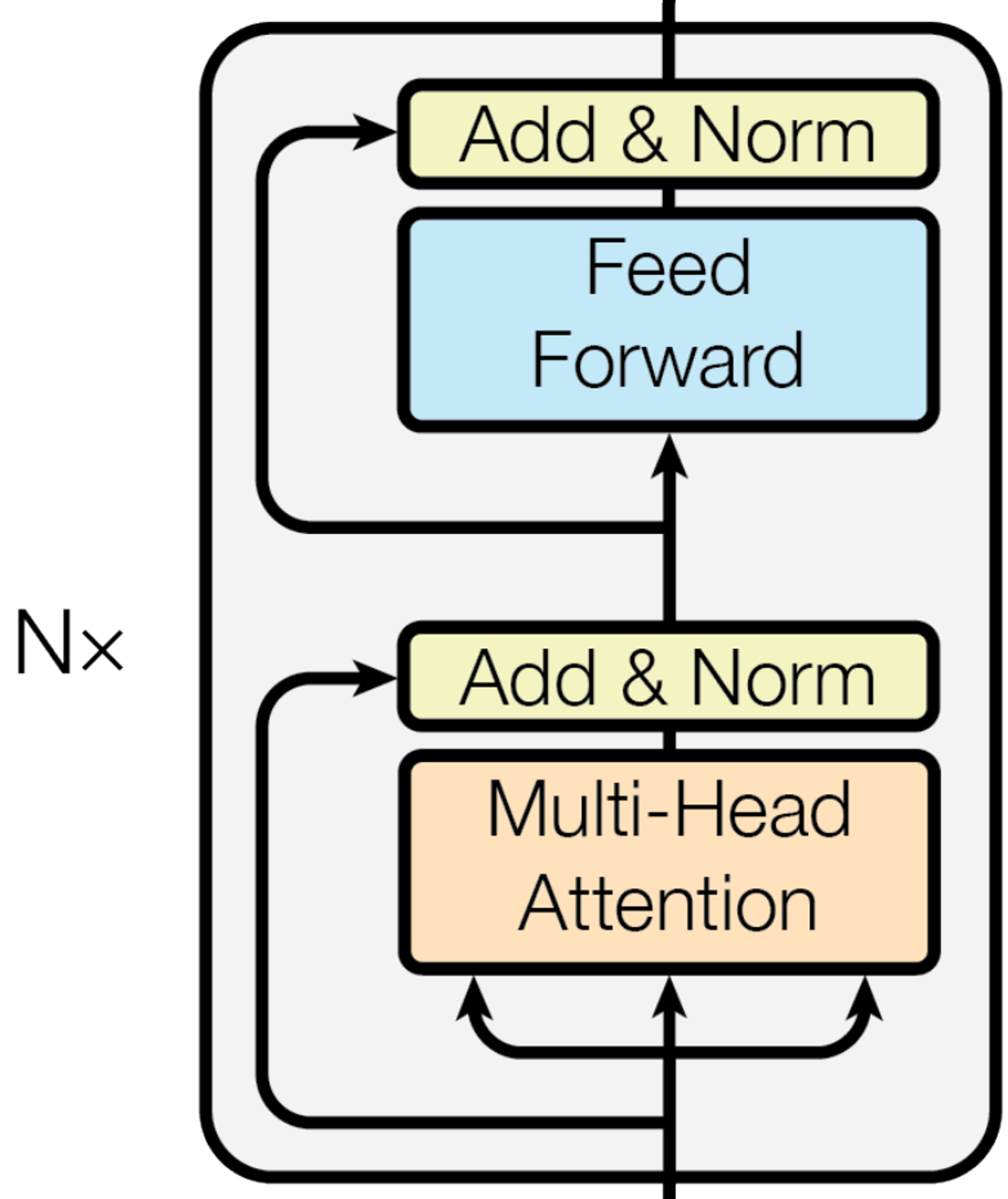
See the "Nx" parts in the architecture diagram?

That simply means the same type of block is applied N times in a row. Each pass refines the representation a bit more.

A good way to think about this is like editing a draft.

• On the first pass, you fix obvious issues.
• On the second, you improve phrasing.
• On the third, you tighten the structure.

Each pass makes the text become clearer and more meaningful every time.

Transformer layers behave the same -- each one builds on the previous, gradually uncovering deeper relationships in the sequence.

Alright, we know we need N such blocks. Let's do that:

class TransformerLayer(nn.Module):
    def __init__(self, d_model: int, n_heads: int):
      super().__init__()

class Encoder(nn.Module):
    def __init__(
        self,
        vocab_size: int,
        d_model: int = 512,
        n_layers: int = 6,
        n_heads: int = 8,
    ):
      self.token_embedding = nn.Embedding(vocab_size, d_model)
      self.transformer_layers = nn.ModuleList(
            [
                TransformerLayer(d_model=d_model, n_heads=n_heads)
                for _ in range(0, n_layers)
            ]
        )

Importantly, we init it through nn.ModuleList to let the optimiser run backward passes on the parameters defined in TransformerLayers.

The first part is the Multi-Head Attention component, which is depicted in the paper as such:

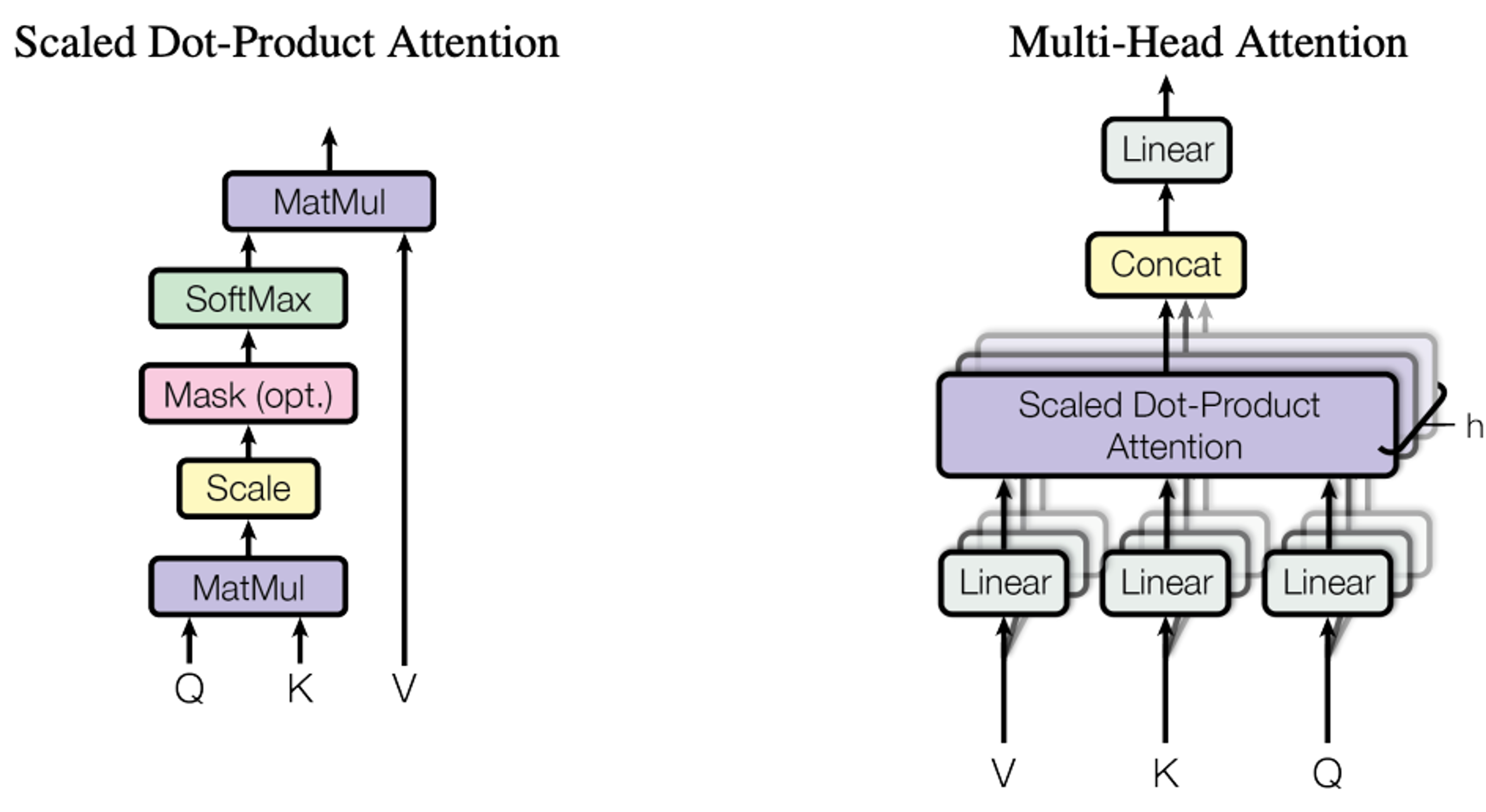
This basically means:

• First, we create h separate attention heads.
• Each head gets its own Query, Key, and Value linear layers.
• The input is sent through every head, where it’s transformed by that head’s Q, K, and V layers.
• We compute attention inside each head by:
  • multiplying Q × Kᵀ to get the attention logits
  • using those logits to weight V, producing the head’s attention output
• After all heads finish, we concatenate their outputs to rebuild the full d_model dimension.
• Finally, the combined output passes through a Feed-Forward Network for additional processing.

We can translate it to code:

class MultiHeadAttention(nn.Module):
    def __init__(self, d_model: int, n_heads: int):
        super().__init__()
 
        self.n_heads = n_heads
        self.d_model = d_model
        self.d_k = d_model // n_heads
        self.Q = nn.Linear(d_model, d_model, bias=False)
        self.K = nn.Linear(d_model, d_model, bias=False)
        self.V = nn.Linear(d_model, d_model, bias=False)
        self.W_O = nn.Linear(d_model, d_model, bias=False)
 
    def forward(self, x: torch.Tensor):
        batch, seq_len = x.size(0), x.size(1)
 
        Q = self.Q(x).view(batch, seq_len, self.n_heads, self.d_k).transpose(1, 2)
        K = self.K(x).view(batch, seq_len, self.n_heads, self.d_k).transpose(1, 2)
        V = self.V(x).view(batch, seq_len, self.n_heads, self.d_k).transpose(1, 2)

We start by defining the Multi-Head Attention class and the Q, K, V projections. In the paper, they suggest each head gets its own Q,K,V. In practice, this would be quite inefficient, because it would require "h" times more matrix multiplications. We can project the inputs once and split them to head chunks to do it in the optimal fashion.

Next, we want to get the attention logits. We need to look at this formula:

Which we can code as such:

        V = self.V(x).view(batch, seq_len, self.n_heads, self.d_k).transpose(1, 2)

        # [batch, d_model, seq_len, seq_len]
        attn_logits = Q @ K.transpose(-2, -1) / math.sqrt(self.d_k)

Remember the chart showing Scaled Dot-Product Attention? We multiplied Q by K, we scaled them with d_k. We are still missing the SoftMax part.

    attn_weights = nn.functional.softmax(attn_logits, -1)

We call it "weights" now, because we have applied a normalisation function over the logits. Now all of the values are normalised -- they sum to 1.

Awesome! Nearly there now. Next part is to multiply attention weights by the Value matrix:

        attention_scores = attn_weights @ V
        attention_scores = (
            attention_scores.transpose(1, 2).contiguous().view(batch, seq_len, self.d_model)
        )

The first line is multiplying tensors of dimension:

• attention weights: [batch, n_heads, seq_len, seq_len]
• V: [batch, n_heads, seq_len, d_k]

Matrix multiplication affects the last two dimensions, so we have:

• [seq_len, seq_len] @ [seq_len, d_k] -> [seq_len, d_k]

So the result is:

• [batch, n_heads, seq_len, d_k]

Now we transpose:

• [batch, n_heads, seq_len, d_k]
• ->
• [batch, seq_len, n_heads, d_k]

and merge the heads:

• ".view(batch, seq_len, self.d_model)"
• [batch, seq_len, n_heads, d_k]
• ->
• [batch, seq_len, d_model]

So in essence we do the "concat" part here.

And the last part is the Feed-Forward network:

    return self.W_O(attention_scores)

That's it! We now have the full Multi-Head Attention module:

class MultiHeadAttention(nn.Module):
    def __init__(self, d_model: int, n_heads: int):
        super().__init__()
 
        self.n_heads = n_heads
        self.d_model = d_model
        self.d_k = d_model // n_heads
        self.Q = nn.Linear(d_model, d_model, bias=False)
        self.K = nn.Linear(d_model, d_model, bias=False)
        self.V = nn.Linear(d_model, d_model, bias=False)
        self.W_O = nn.Linear(d_model, d_model, bias=False)
 
    def forward(self, x: torch.Tensor, padding_mask: torch.Tensor | None = None):
        batch, seq_len = x.size(0), x.size(1)
 
        Q = self.Q(x).view(batch, seq_len, self.n_heads, self.d_k).transpose(1, 2)
        K = self.K(x).view(batch, seq_len, self.n_heads, self.d_k).transpose(1, 2)
        V = self.V(x).view(batch, seq_len, self.n_heads, self.d_k).transpose(1, 2)
 
        # [batch, d_model, seq_len, seq_len]
        attn_logits = Q @ K.transpose(-2, -1) / math.sqrt(self.d_k)
 
        attn_weights = nn.functional.softmax(attn_logits, -1)
 
        attention_scores = attn_weights @ V
        attention_scores = (
            attention_scores.transpose(1, 2).contiguous().view(batch, seq_len, self.d_model)
        )
 
        return self.W_O(attention_scores)

We're on the finish line now. We just need to stitch it all back together and add the FFN and Add & Norm components to our Transformer block.

First, the Add & Norm. We can get it with a pre-existing PyTorch module:

class TransformerLayer(nn.Module):
    def __init__(self, d_model: int, n_heads: int):
        super().__init__()
 
        self.layer_norm_1 = nn.LayerNorm(d_model)
        self.layer_norm_2 = nn.LayerNorm(d_model)

And a method to perform the addition and normalisation:

    def add_and_norm(self, layer_norm: nn.LayerNorm, input: torch.Tensor, x: torch.Tensor):
        added = torch.add(input, x)
        return layer_norm(added)

Then, we define the FFN:

        # Second sub-layer is a position-wise fully connected feed-forward network
        self.FFN = nn.Sequential(
            # defaults will be 512 -> 2048, same as in the paper
            nn.Linear(d_model, d_model * 4),
            nn.ReLU(),
            nn.Dropout(0.1),
            nn.Linear(d_model * 4, d_model),
        )

Notice I mixed in the nn.Dropout, since it's a very powerful regularisation technique. It helps achieve good generalisation.

Now stitch it back together:

class TransformerLayer(nn.Module):
 
    def __init__(self, d_model: int, n_heads: int, dropout_proba: float):
        super().__init__()
 
        self.dropout_proba = dropout_proba
 
        self.layer_norm_1 = nn.LayerNorm(d_model)
        self.layer_norm_2 = nn.LayerNorm(d_model)
 
        # As per paper, we implement two sub-layers.
        # First is a multi head self attention layer
        self.multi_head_self_attn = MultiHeadAttention(d_model, n_heads, dropout_proba)
 
        # Second sub-layer is a position-wise fully connected feed-forward network
        self.FFN = nn.Sequential(
            # defaults will be 512 -> 2048, same as in the paper
            nn.Linear(d_model, d_model * 4),
            nn.ReLU(),
            nn.Dropout(dropout_proba),
            nn.Linear(d_model * 4, d_model),
        )
 
    # x should be of shape [batch, seq_len, d_model]
    def forward(self, x: torch.Tensor, padding_mask: torch.Tensor | None = None):
        # From the paper:
        # MultiHead(Q, K, V ) = Concat(head1, ..., headh)W^O
        multi_head_attn_out = self.add_and_norm(
            self.layer_norm_1,
            self.multi_head_self_attn(x, padding_mask=padding_mask),
            x,
        )
 
        # Feed-forward network
        block_out = self.add_and_norm(
            self.layer_norm_2,
            self.FFN(multi_head_attn_out),
            multi_head_attn_out,
        )
 
        return block_out
 
    def add_and_norm(self, layer_norm: nn.LayerNorm, input: torch.Tensor, x: torch.Tensor):
        added = torch.add(input, x)
        return layer_norm(added)

And finally, our Encoder is complete:

class Encoder(nn.Module):
 
    def __init__(
        self,
        vocab_size: int,
        d_model: int = 512,
        n_layers: int = 6,
        n_heads: int = 8,
    ):
        super().__init__()
 
        self.d_model = d_model
        self.token_embedding = nn.Embedding(vocab_size, d_model)
        self.transformer_layers = nn.ModuleList(
            [
                TransformerLayer(d_model=d_model, n_heads=n_heads)
                for _ in range(0, n_layers)
            ]
        )
 
    def forward(self, token_ids: torch.Tensor):
        embeddings = self.token_embedding(token_ids)
 
        embeddings = embeddings * math.sqrt(self.d_model)
 
        pos_encoding = self.get_pos_encoding(embeddings)
        out = embeddings + pos_encoding
 
        for layer in self.transformer_layers:
            out = layer(out)
 
        return out

That concludes it!

We now have the full Transformer Encoder implemented.

It was not an easy ride, and I had to omit a few details to prevent this post from getting too long. In practice we'd also include a few more things, like dropout to attention out or padding mask.

All in all it was a really fun exercise, and I hope you enjoyed the ride along.

Feel free to browse the entire code on my github. It contains the few additional pieces I omitted for the purpose of simplification.

Thank you!